|

|
|
I. Introduction: Nonlinear Dynamical Systems
- Dynamical systems described by differential equations
a. Example: Newton's 2nd Law
b. Uniqueness
c. Linear and nonlinear superposition
d. analytic solutions not always possible
- Archetypal Example: the plane Pendulum
a. Energy integral
b. Exact, implicit solution
c. Phase Portrait (from energy integral) and orbit types
d. Equilibrium (fixed) points and stability (elliptic and hyperbolic)
e. Addition of Damping: spiral ( focus ) fixed points and basins of attraction
f. Addition of driving force: extended phase space, no more fixed points,
complicated motion
- Some basic ideas: dynamical systems and the geometry of phase space
a. ODE Dynamical System:  for i = 1, N
( N = dimension of phase space )
b. Solution: a trajectory ( dimension 1 ) , one for each initial condition
c. Integrals of motion: function  =
constant =
constant
d. Integrals of motion confine the motion to a "surface" in phase space
and reduce effective phase space dimension by 1.
e. Trajectory can be thought of the intersection of all the Integral surfaces;
therefore need N - 1 integrals of motion to completely solve
for a trejectory.
f. If well behaved integrals of motion don't exist the system is nonintegrable
( more later )
- Fixed Points and Stability
a. Fixed point of ODE Dynamical System: a point where
= 0 for all i = 1, N
b. For system obeying Newton's 2nd Law: velocity and acceleration vanish
- i.e. a point of local equilibrium.
c. Stability: Linearize about the fixed point  where
where  and form the stability matrix M = Jacobian of the set of ODE's. Eigenvalues
 of
M determine stability. of
M determine stability.
d. Lyapunov Stability Theorem: If, at fixed point  for all i, then x* is stable. Otherwise x* is unstable.
e. Fixed Points in 2-d:
- Both eigenvalues imaginary => center ( elliptic ) fixed point (
not unstable )
- Both eigenvalues real, < 0 => stable node ( or star if
 )
)
- Both eigenvalues real, > 0 => unstable node ( or star if
)
- Both eigenvalues real, opp. sign => saddle ( hyperbolic ) fixed
point ( unstable )
- Both complex, Re ( )
< 0 => stable focus ( spiral )
- Both complex, Re (
) > 0 => unstable focus ( spiral )
f. Potential functions and Turning Points:
- For conservative Newtonian system the minima of the potential are elliptic
fixed points and the maxima are hyperbolic fixed points. Separatrix curves
pass thru the hyperbolic points. Turning points are positions where total
energy E = V = potential. Use these facts to sketch phase portrait
from potential.
g. Nonautonomous ( explicitly time dependent ) systems:
- Define extended phase variable
 ,
where ,
where  = constant and t = time.
- Increases phase space dimension by 1, but now treat the system as autonomous.
- Lagrangian Dynamics
a. Generalized coordinates and velocities
b. Lagrangian function L = T - V and Euler-Lagrane equations
of motion
c. Ignorable coordinates: If L is independent of  then the conjugate generalized momentum
  is conserved: useful method for finding an integral of motion.
d. If L is independent of t then  is conserved
e. H = Hamiltonian is equal to E only if the equations transforming
rectangular coordintes to generalized coordinates are time independent and
the potential V depends only on the coordinates. In this case H =
E = T + V
- Hamiltonian Dynamics
a. Natural variables for H are the  's
and the 's
("canonical" variables). 's
and the 's
("canonical" variables).
b. Hamilton's equations of motion: 
c. Ignorable coordinates, same as for L : If H is independent
of
then the conjugate momentum
is conserved. If H is independent of t then H is conserved
d. Symmetry and conservation laws:
- translational symmetry => conserved momentum
- rotational symmetry => conserved angular momentum
- time translation.symm. => conserved H ( energy )
- Integrability
a. A Hamiltonian system of dimension N = 2n is integrable
if there exist n global, single valued integrals of motion which
are in involution.
b. Note difference from general dynamical system which requires N
- 1 integrals to be integrable.
c. "In involution" means pairwise Poisson brackets vanish.
d. "Most" Hamiltonian systems are nonintegrable ( the integrable ones
are a set of measure zero )
e. Liouville's Theorem: Volumes in phase space are preserved by Hamiltonian
flows.
- Poincaré Surface-of-Section ( SOS )
a. Most useful for 3-D phase space ( or higher if it can reduced to 3 with
integrals of motion )
b. Choose convenient surface in phase space and plot point each time the
orbit passes through that surface with one velocity direction.
c. Orbit types:
1. Regular ( periodic and quasiperiodic ): smooth curves or single dot
2. Chaotic: "random" dots filling a region of larger dimension than
1.
3. Transient: Orbits which interact for a finite time, then leave forever:
finite sequence of dots ( can appear chaotic, so you must look at individual
orbits to tell )
d. Separation of regular and chaotic regions: determine the structure
of phase space
- Physics Example: Charged Particles in Magnetic Neutral Lines
a. SOS plots show hyperbolic fixed point with stable and unstable manifolds
( "SUM" ), even in chaotic region.
b. SUM divides region of phase space where orbits pass through x
= 0 from region where orbits do not pass thru x = 0.
c. Statistical orbit studies show "ridge" in velocity distribution function
caused by the same orbit separation: the ridge is due to the SUM in phase
space.
d. Spacecraft observations seem to confirm the existance of ridges near
the center of the current sheet in the earth's magnetotail at the onset
of an auroral substorm.
- Chemistry Example: Molecular Binding in ABA triatomic molecules
a. Use Morse potential to describe bonds
b. Derive Hamilton's equations and produce SOS plots: fixed points corresponding
to local ( one bond vibrating ) and normal ( both bonds vibrating ) modes
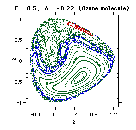
c. Bond-selective chemistry: excite local mode and favor one of several
possible routes for reaction. e.g. H + HOD ->  + OD or H + HOD -> HD + OH; laser excite the local H-O mode in HOD and
the H-O bond breaks, favoring the first reaction. Recently observed in experiments.
+ OD or H + HOD -> HD + OH; laser excite the local H-O mode in HOD and
the H-O bond breaks, favoring the first reaction. Recently observed in experiments.
d. Chaos appears as energy or bond coupling increases. More chaos means
that energy is ditributed rapidly throughout the molecule, so bond-selective
chemistry is less likely. Also, because chaotic vibrations cannot be classified
as local or normal, it is difficult to assign good quantum numbers to the
transitions and therefore more difficult to interpret spectra.
- KAM Theory
a. Simple perturbation theory: approximate solutions expanded in terms
of a small parameter.
b. Action - Angle variables: New generalized variables where all momenta
are integrals of motion ( for an integrable system )
c. New momenta:  ("action");
new coordinate: ("action");
new coordinate:  ( "angle" )
d. Canonical perturbation theory uses action-angle variables. In 1-d,
the perturbed action is 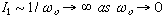 as
as  -> 0; i.e. zero oscillation frequency ( like pendulum near hyperbolic
fixed point and separatrix ) causes expansion to fail: the problem of
small divisors
-> 0; i.e. zero oscillation frequency ( like pendulum near hyperbolic
fixed point and separatrix ) causes expansion to fail: the problem of
small divisors
e. Higher dimensions: n angles and n constant actions =>
motion on an n-torus.
resonant ( or rational ) tori:  for integer
  's
( frequencies are commensurate ); corresponds to periodic orbits 's
( frequencies are commensurate ); corresponds to periodic orbits
nonresonant ( or irrational ) tori: no set of integers  satisfying
above eqn. ( frequencies incommensurate ); corresponds to quasiperiodic
orbits satisfying
above eqn. ( frequencies incommensurate ); corresponds to quasiperiodic
orbits
f. KAM Theorem: If H is analytic in some finite region and
the system is nondegenerate then tori with ( for n = 2 only ) 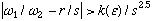 (
where r and s are integers and k
is a constant for each (
where r and s are integers and k
is a constant for each  are preserved under perturbation of size .
Note resonant tori are not preserved, but tori with "far from rational"
frequency ratio are preserved. Destruction of tori correspond to the onset
of chaotic orbits, preservation of tori means regular motion is preserved
under the perturbation.
are preserved under perturbation of size .
Note resonant tori are not preserved, but tori with "far from rational"
frequency ratio are preserved. Destruction of tori correspond to the onset
of chaotic orbits, preservation of tori means regular motion is preserved
under the perturbation.
g. Poincaré - Birkhoff Theorem: Under perturbation a resonant
torus breaks up into alternating elliptic and hyperbolic fixed points (
and chaos ), with ( # of elliptic f.p.'s ) = ( frequency ratio of resonant
torus which breaks up ).
- The Chaotic Hierarchy
a. Ergodic system: single orbit visits all accessible phase space
b. Mixing system: systems with SIC: at least 1 positive Lyapunov exponent.
Mixing systems have continuous power spectrum.
c. K-system: has positive Kolmogorov entropy, i.e. positive average divergence
rate
d. C-system or Anusov: All Lyapunov exponents are positive. Implies
- tracing property which justifies numerical computation in chaotic systems:
the numerical orbit will be within
of some orbit in the system.
e. Bernoulli system: "as random as a coin toss"
- Can Irreversibility be derived from Reversible Microphysics?
a. What makes time go forward? Microphysical theories are reversible (
Newton's laws, Schroedinger equation, etc. )
b. Does chaos imply irreversibility? Chaos leads to diffusion in phase
space which could imply a direction of time.
c. Kubo formula relates diffusion coefficient ( irreversible ) to velocity
auto-correlation function C ( t ) ( computed with reversible dynamics ).
d. Results for Lorentz gas ( periodic array of scatterer disks with point
particle bouncing around ): (1) If there are infinite free paths between
scatterers then  ( non-diffusive ) but (2) If there are no infinite free paths then
  ( diffusive ). Conclusion: even this strongly chaotic system cannot guarantee
irreversibility.
( diffusive ). Conclusion: even this strongly chaotic system cannot guarantee
irreversibility.
- Attractors
a. Dissipative systems characterized by attractors: sets ( typically
of lower dimension than the full phase space ) into which orbits are attracted
as time  . .
b. Examples of attractors: attracting fixed points, limit cycles, tori,
and "strange".
c. Basin of attraction of an attractor: That subset of phase space which
maps asymptotically ( i.e. as
) into the attractor. A system can have multiple attractors each with mutualy
exclusive basins of attraction.
- Limit Cycles and Poincaré - Bendixson Theorem
a. A limit cycle is a closed periodic orbit - it can either be attracting
or repelling.
b. Poincaré - Bendixson Theorem: If a solution x(t) to dynamical
system stays in some region K as ,
then K must contain at least one fixed point or a periodic orbit ( i.e.
a limit cycle )
c. Van der Pol oscillator circuit: nonlinear circuit with limit cycle
for parameter e between zero and 2.
- Bifurcations
a. A bifurcation value of a parameter is a value at which the flow is not
structurally stable; i.e. at the bifurcation point the behavior of the system
changes to one which is not topologically equivalent to the original flow.
b. Saddle-node ( tangent ) bifurcations: no fixed points bifurcate into
1 stable and one unstable fixed point ( a saddle and a node in 2-d ).
c. Transcritical bifurcation: one stable and one unstable "change places"
d. Pitchfork bifurcation: One stable fixed point bifurcates into one unstable
and two stable fixed points.
e. Hopf bifurcation: One stable fixed point bifurcates into one unstable
fixed point and a limit cycle ( e.g. Van der Pol oscillator ).
- Archetypal Example: The Lorenz Model
a. Originally a simplification of the Navier-Stokes fluid equations, resulting
in 3 first-order ODE's. Many related systems in other fields.
b. Stability analysis shows pitchfork bifurcation followed by homoclinic
bifurcation followed by inverse Hopf bifurcation: interpreted as onset of
convection ( pitchfork ), onset of transient chaos ( homoclinic ), chaotic
strange attractor implying turbulence ( between homoclinic and Hopf bifurcations
), and the disappearance of all stable motion ( Hopf bifurcation ).
c. Even more complex behavior for larger values of the parameter: intermittency
and crises.
d. Lorenz map: look a maximum of one variable at a plane in phase space,
and the system can be reduced to a 1-d map.
- Approaches to Chaos
a. Period doubling cascade ( pitchfork bifurcation )
b. Intermittency ( tangent bifurcation )
c. Crises ( unstable branch of tangent bif. "collides" with period doubling
cascade )
d. Quasi-periodic or Ruelle-Takens: Hopf bifurcations producing a few
discrete frequencies, then chaos.
e. Use to model the approach to turbulence in fluids. All approaches are
observed in experiments.
- Fractals
a. Chaotic attractors often have complex geometric structure showing structure
on all spatial scales. This is characteristic of fractal objects: objects
with fractional dimension.
b. Box counting Dimension: 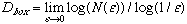 ,
where N (
) = number of boxes of size
needed to cover the attractor. ,
where N (
) = number of boxes of size
needed to cover the attractor.
c. Example: Cantor set,  = ln2 / ln3
d. Example: Koch snowflake,
= ln4 / ln3
e. Phase space reconstruction: reconstruct higher dimensional attractor
from only one time series of data. Use time-delay coordinates (  is a constant time delay )

f. Choice of
is critical for the method to work.
g. Correlation Dimension: compute correlation sum
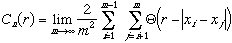
for several embedding dimensions. Find slope of "scaling region" of log-log
plot of  (r)
vs. r ( i.e. that part which is a power law ) and plot slope vs embedding
dimension. If a limit is reached then (r)
vs. r ( i.e. that part which is a power law ) and plot slope vs embedding
dimension. If a limit is reached then  =
the limiting slope. If no limit, then the data is random. =
the limiting slope. If no limit, then the data is random.
h. Caveats for :
use embedding dimension 
 + 1; need at least
  data points in the timeseries; beware of "colored noise" which can imitate
this limiting behavior.
data points in the timeseries; beware of "colored noise" which can imitate
this limiting behavior.
i. Example
- Physics/Engineering Example: The bouncing ball electronic circuit
a. demonstrated in class: can observe both periodic and apparently chaotic
behavior; phase portraits, power spectra, and Correlation dimension apparently
discriminate between regular, chaotic, and random motion;
~ 1.7 for chaotic attractor.
- Utility of :
Reduction of Dimension with Strange Attractors:
a. Relation of
to other quantities:
b. Reduction of Dimension: Number of independent variables need
to describe the attractor is  2
+ 1. So if high-dimensional system has a strange attractor, it can be possible
to study it using lower dimensional models.
2
+ 1. So if high-dimensional system has a strange attractor, it can be possible
to study it using lower dimensional models.
c. Example: B-Z Reaction: FKN reaction mechanism has 15 reactants, yet
SOS plot made from reconstructed attractor allows study as 1-d map.
d. Example: Couette-Taylor fluid flow; turbulent state has infinite number
of degrees of freedom ( Fourier frequencies, e.g. ), but
~ 3.1, so the system can ( in principle ) be studied with between 4 and
2(4)+1 = 9 variables.
e. Example: Auroral Substorms using the AE index; there is no good theoretical
model, so the number of degrees of freedom is large, but unknown. After
removing input (solar wind) noise with singular spectrum analysis, get
~ 2.5, so between 3 and 7 variables are needed to describe the system. Attempts
to model the magnetosphere as an electronic circuit have been somewhat successful.
f. Knowing that the system is low dimensional and finding the relevant
variables are two different things. There is a mathematical procedure that
can define a set of variables, but it is nontrivial and the results are
not easily interpretable physically.
- Stretching and Folding: Baking and Horseshoes
a. Pastry maps: stretch the dough then fold it over, repeat. After an infinite
number of iterations this yields a Cantor-like structure.
b. Baker's Map: cut the dough in center after stretching, then layer.
Leads to
= 1-ln2 / ln ,
where
= height reduction factor during the stretch. Can represent the map as a
binary shift and prove it's equivalent to a coin toss. Thus it has a strange
attractor.
c. Smale's Horseshoe: Fold the dough first then stretch, then cut off
any that hangs over the interval [0,1]. This has similar fractal properties
to Baker's map but is not chaotic ( as
), so it is a nonchaotic strange attractor ( but it exhibits transient chaos
for finite times ).
d. Many strange attractors have Horseshoe behavior "in them" - the trick
is to discover how. Examples were given of Lorenz, Rossler, and Hénon
map, and standard map models of strange attractors.
e. Also there is a Horseshoe in every unstable hyperbolic point, even
for Hamiltonian systems, due to Homoclinic orbits. So chaos seems to be
related to Horseshoes.
- Control of Chaos
a. Logistic map example: near unstable fixed point, if vary the parameter
 at each iteration we can keep the orbit bounded, and keep the system stable.
b. C-Feedback Example: Extension of cubic autocatalator model ( which
had a limit cycle for some parameters ) which exhibits chaos; by SOS technique,
it can be reduced to a 1-d map; study the map for different parameter values
and control to eliminate chaotic behavior.
c. Experimental example: Using B-Z reaction, do computer simulation to
estimate the control mechanism, then try actual experiment, which is successful.
d. 2-d systems: Look at stable and unstable manifolds of an unstable fixed
point; find the effect of varying a system parameter, and select the variation
which puts the iterate on the stable manifold of the original map; example
cardiac chaos.
- Symmetry and Complexity
a. Use mathematical symmetries to simplify calculations; physical symmetry
to simplify physical models; physical symmetries to find conservation laws
( Noether's Theorem ).
b. Thermodynamic equilibrium is a highly symmetric state.
c. Symmetry is "boring":
spatial symmetry => lack of spatial structure ( shape and form ),
temporal symmetry => lack of past and future
equilibrium => nothing happens at all
d. Real world is complex: characterized by constant change, spatial structure,
pattern formation, evolution of more complexity, etc. => How?
e. Complexity properties: dissipative, nonlinearities important, nonequilibrium,
long-range order.
f. Bénard fluid system example: Experimenter breaks vertical symmetry
by establishing ( nonequilibrium ) temperature gradient. System spontaneously
breaks horizontal symmetry when convection begins. Dependent on ( random
) fluctuations and nonlinearities in the system. Interplay of random
fluctuations and nonlinearites produce long-range order.
g. Simple model: pitchfork bifurcation; symmetry-braking bifurcations
generate structure.
h. Laser Example: Use adiabatic approximation ( "the slaving principle":
Long-living systems slave short-living systems ) to elicit the basic structure
of symmetry-breaking bifurcation leading to lasing. Same behavior for many
other systems with multiple timescales.
- Spatio-temporal Pattern Formation and Cellular Automata
a. Spatial structure typically requires PDE's - beyond the scope of this
course.
b. Cellular Automata ( CA ) provide an alternate approach: A CA is given
by a set of cells, an integer function  which assigns an integer value to each cell at generation n, and a set of
rules which advance the function values for each cell by one generation:
which assigns an integer value to each cell at generation n, and a set of
rules which advance the function values for each cell by one generation:
 . .
c. Example: 1-d Game of Life: N cells with X( i )
= 1 ( for alive ) or 0 ( for dead ); rules specify live cell with live neighbors
dies, dead cell with live neighbors is born, live cell with dead neighbors
dies. Results with periodic boundary conditions are all initial states lead
to extinction for odd N, periodic solutions possible for even N.
For higher dimension you can get chaos as well.
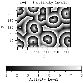
d. Example: Greenberg-Hastings Model: 2-d system of cells, with
rules involving r -neighbors; can result in complex pattern formation, similar
to patterns seen in B-Z reaction in a shallow dish.
- Models and Paradigms
a. Are continuous models always the best? ( There are well-know problems
with continuous models; e.g. infinities and renormalization ) Or should
we consider manifestly discrete models ( like Caldirola, T. D. Lee, general
relativity, etc ).
b. Historical "analytic" paradigm has science discovering building blocks;
more recent "synthetic" approach discovers synergy of building blocks and
emergent properties: the whole is more than the sum of its parts.
- Self-Organized Criticality and Sandpiles
a. 1-d Sandpile CA yields attracting stationary state at maximum instability:
add more sand and it falls down the slope; remove some and the sand above
falls down.
b. 2-d Sandpile CA yields self-organized critical state, where domain
of influence of a perturbation can cover any scale size.
c. May be a paradigm for emergent properties and pattern formation.
![[bullet]](../../images/greenball.gif) Go back
to Computational Science Courses Go back
to Computational Science Courses
Go to Current
Molecular Dynamics Course
|
|


