Apparatus, Data Taking, and Data Analysis

The first working version of the ISU waterwheel is shown below, and many of its features carry over into the latest version.

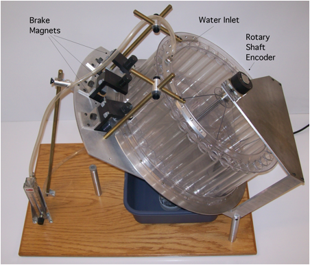
The wheel consists of a polycarbonate base on which are mounted 36 polycarbonate cylinders on a circle with 18 in diameter.  The base includes a cone shaped depression over which each cylinder is mounted.  A hole is drilled in the bottom of each cone to accept a nylon screw, and a small diameter (about 0.04 in) hole is drilled in the length of each screw (about 1 in) to allow the water to leak from each cell.  A vacuum-formed trough is attached to the tops of the cylinders to ensure that all the incoming water stream is directed into the cells.  A trough under the wheel collects the water and returns it to the reservoir.  Roller bearings support the shaft above and below the wheel and allow free rotation.  An optical rotary encoder is attached to the upper end of the shaft to record angular position data.  An annular ring of thin aluminum is attached to the base of the wheel and passes between the pole faces of a variable gap magnet.  This produces a braking torque that varies almost linearly with the angular velocity.  Water enters at the very top of the wheel in a single stream, although other angular distributions are possible.  The data currently presented on this website were acquired with this arrangement of the apparatus.

Shown below is the current version of the apparatus. 

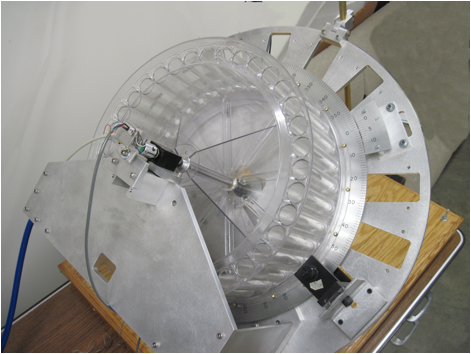
The water inlet is not shown in this picture.  A much more robust frame is now used to provide the necessary stiffness for mounting of air bearings, which have replaced the roller bearings.  Also, the aluminum ring has been replaced by a duplicate with precision angular markings that, with the vernier scale, give 0.1 degree absolute accuracy to the wheel’s position.  This is necessary to provide calibration of the non-contact two-axis Hall sensor used to measure the wheel’s angular position (see figure below).

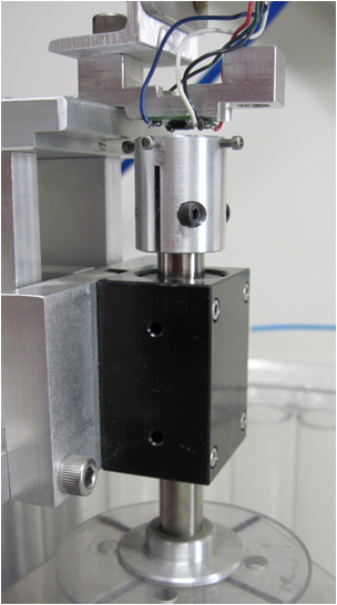
The dark block is the cylindrical air bushing that holds the top of the wheel’s shaft.  The aluminum cylinder at the top of the shaft holds a small, square, rare earth magnet with magnetization in the horizontal plane.  Just above the magnet is the two-axis Hall sensor, which gives voltages Vx and Vy that are proportional to the component of the magnetic field in those directions.  Very small nonlinearities in the sensor’s response must be removed to achieve greatest accuracy; hence the reason for the fixed angular scale around the wheel’s edge.

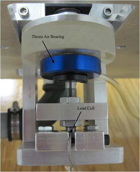
In addition, the wheel rests on a single “hockey puck” style air bearing that assumes the thrust load that the two air bushings cannot support.  To monitor the amount of water in the wheel, we have also mounted a load cell under the thrust bearing.  Both are shown in the picture below.

Setting the Parameters

The tilt angle of the wheel (typically around 42 degrees) and the input water flow rate (typically around 26 gal/hr or about 0.027 kg/s) are easily set and measured.  The braking parameter requires a little more effort to measure.  After setting the magnet gap spacing (sometimes multiple magnets are used), the wheel is given a spin and angular data are acquired while the wheel slows down.  Then, assuming the braking torque is, one can fit the resultant data to the general form of the solution and extract the parameter ratio , which we typically call C.  This parameter is determined with no water in the wheel, and we call that reference value C0.  This parameter is currently used as our bifurcation parameter.

Acquiring and Analyzing the Data

The empty wheel is given a small initial velocity and the water is allowed to enter the wheel.  After a delay of at least 15 minutes, we begin to acquire time-stamped angle data, with a time spacing around 0.025 s.  We then use Mathematica to interpolate the data (allowing us to correct the small non-uniformity in the time spacing of the raw data) and apply a fast Fourier transform to the data.  We then calculate the necessary derivatives in Fourier space, remove frequency components above a cut-off frequency (typically around 0.5 Hz), then recreate the smoothed data via inverse Fourier transform.

The Future

The new wheel has several advantages over its predecessor.  The air bearings have reduced mechanical friction to its practical minimum, which may correct some of the deviations we see between the wheel’s behavior and the predictions of the model equations.  The load cell allows us to investigate whether the mass of the wheel varies during its motion, and preliminary evidence suggests that it does.  The previous data were taken with an optical rotary encoder attached to the wheel’s shaft, while the new setup utilizes a non-contact two-axis Hall sensor to measure the angle.  We now must recreate the large array of data produced with the first setup and then continue to explore the vast parameter space of this rich dynamic system.